HTS Modelling Workgroup
Research on modelling tools is a fundamental topic in applied superconductivity
HTS materials raise complex challenges in the design and prediction of devices' behavior due to i) the strong coupling between their nonlinear and anisotropic electromagnetic and thermal properties, and ii) the high aspect ratio of HTS tapes. State-of-the-art research in HTS modelling tools consider this reality and propose ways to address these challenges. Many examples are provided on this website.
HTS modelling website and workshops
In the last 20 years, numerical modelling has become widely adopted as the most powerful tool for research and development of High Temperature Superconductor (HTS) applications. Several groups around the world have worked on the development and the testing of various models and numerical techniques. A better communication channel between the researches and engineers had to be put in place in order to speed up the collective advances and to limit work duplication.
The first step in this direction was taken in 2010, with the organization of the first International HTS modelling workshop in Lausanne, Switzerland. The large number of attendees and the positive feedback led to the organization of other workshops in the following years (see the Workshops tab for more details).
During these workshops, many participants recognized the need of having a permanent platform on the internet for facilitating exchanges between researchers and accessing up-to-date information on the latest developments. The aim of this website is to be that platform. Please browse through the tabs above ro access the different pages of this website, and do not hesitate to contact us for comments and suggestions.

Special Session on Numerical Modeling of HTS at EUCAS 2025
Archive Hall (1200)
Porto, Portugal

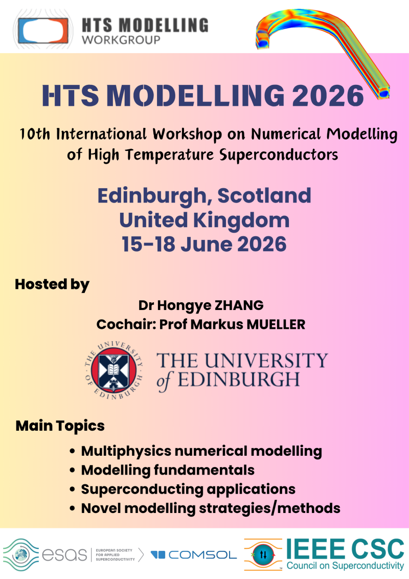
10th International Workshop on Numerical Modelling of High Temperature Superconductors
June/July, 2026
Edinburgh, Scotland United Kingdom
