Special Session on Numerical Modeling of HTS at EUCAS 2025
Special Session
Special Session on Numerical Modeling of HTS at EUCAS 2025
Special Session of EUCAS 2025
Archive Hall (1200)
Archive Hall (1200)
Monday, September 22, 14:30 – 16:00
Porto, Portugal

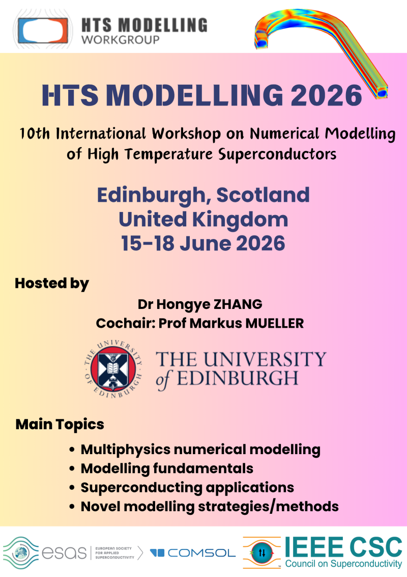
10th International Workshop on Numerical Modelling of High Temperature Superconductors
Workshop
10th International Workshop on Numerical Modelling of High Temperature Superconductors
June/July, 2026
Edinburgh, Scotland United Kingdom